
ABEJAアドベントカレンダー2025の24日目の記事です。
ABEJAでデータサイエンティストをしている大谷です。
最近VLAに触れ合うことが増えてきました。11/7にもMacStudioで動かすSO-ARM x π0.5 -解説から実機動作まで-というタイトルで登壇もしました。
ただ、この登壇の時にも感じたのですが、π0で採用されているaction expertが完全理解に至っていないです。
というわけで今回のブログではopenpiの実装からaction_expertの部分に絞ってコードレベルで見ていくことで理解を深めていきます。
πシリーズとは
π0から始まったπシリーズ(勝手にシリーズと呼んでいます)は、Physical Intelligence 社が開発した VLA モデルです。 手前味噌で恐縮ですが、π0の仕組みは弊社のテックブログを参考にいただける幸いです。
https://arxiv.org/pdf/2410.24164arxiv.org
その後、π0.5、π*0.6と続きます。後続モデルでもaction expertは使用されています。
https://arxiv.org/pdf/2504.16054arxiv.org
action expertとは
ざっくり連続したアクション生成をするために、VLMモデルに追加された部分です。ロボットはアームの回転角制御など可能な限り細かい周期で連続的に操作していきたいです。ただ出力するactionがVLMの出力速度にピン留めされてしまうと、ロボットの制御がカクついてしまいます。そこでaction expertをVLMの外に後付けし、高精度の連続アクション分布をFlow Matchingで生成することで、高い周波数での制御値を連続値として出力できるようにしました。
ちなみにFlow Matchingもわかるようでわかっていないことが多いので、ここも合わせてコードで理解していこうと思います。
Flow Matchingはざっくりいうと、適当な確率分布(ノイズ分布など)から欲しい確率分布まで、徐々に意味のある滑らかな動きに変化させる技術です。ロボットでいうとノイズから正解のアクションへ向かう中間アクションを学習する感じです。
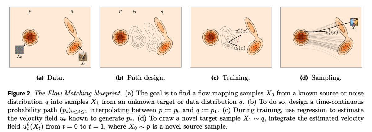
https://arxiv.org/pdf/2412.06264arxiv.org
サンプルデータでFlow Matchingを試す
Flow Matching Guide and CodeのP7にサンプルコードがあるので、これを使って基礎から理解します。
import torch
from torch import nn, Tensor
import matplotlib.pyplot as plt
from sklearn.datasets import make_moons


class Flow(nn.Module):
    def __init__(self, dim: int = 2, h: int = 64):
        super().__init__()
        self.net = nn.Sequential(
            nn.Linear(dim + 1, h), nn.ELU(),
            nn.Linear(h, h), nn.ELU(),
            nn.Linear(h, h), nn.ELU(),
            nn.Linear(h, dim)
        )

    # x_t: (B,2), t: (B,1)
    def forward(self, x_t: Tensor, t: Tensor) -> Tensor:
        return self.net(torch.cat((x_t, t), dim=-1))

    # simple midpoint ODE solver step
    def step(self, x_t: Tensor, t_start: float, t_end: float) -> Tensor:
        t_start_tensor = torch.full((x_t.shape[0], 1), t_start)
        t_end_tensor   = torch.full((x_t.shape[0], 1), t_end)

        dt = t_end - t_start

        # midpoint method
        k1 = self.forward(x_t, t_start_tensor)
        x_mid = x_t + 0.5 * dt * k1
        t_mid = torch.full((x_t.shape[0], 1), (t_start + t_end) / 2)
        k2 = self.forward(x_mid, t_mid)

        return x_t + dt * k2
モデル定義は超シンプルですね。step関数ではx_tをt_startからt_endまで1ステップ分移動させます。
dt = t_end - t_startで時間の幅を計算し、その速度(傾きの方が正しい?)k1をモデルで予測。
速度k1を使って時間が半分だけ進んだ場所(0.5 * dt)を計算し、x_midを算出。中点x_midと中間時刻t_midを使ってもう一度速度を予測して誤差を減らしています。(中点法)
最後に中点で求めた速度k2でx_tからdt分移動した最終的な位置を返すといった処理です。
言われてみればまぁそうだよね、という感じです。 それでは以下のようなノイズからいつもの三日月を予測していきましょう。
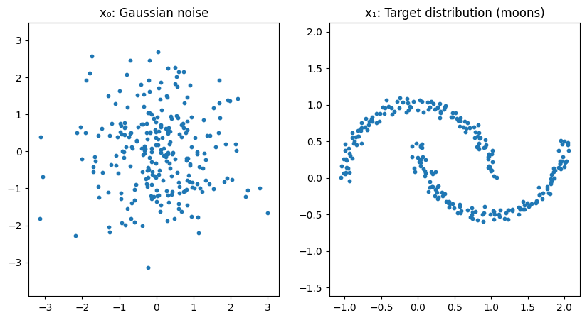
# モデルを定義
flow = Flow()
optimizer = torch.optim.Adam(flow.parameters(), lr=1e-2)
loss_fn = nn.MSELoss()


# 学習
for step in range(10000):
    # いつも三日月(ターゲット)
    x_1_np, _ = make_moons(256, noise=0.05)
    x_1 = torch.tensor(x_1_np, dtype=torch.float32)
    # ノイズ
    x_0 = torch.randn_like(x_1)

    # x_1とx_0を直線で結ぶ
    t = torch.rand(len(x_1), 1)
    x_t = (1 - t) * x_0 + t * x_1
    # 正解の速度ベクトル
    dx_t = x_1 - x_0

    optimizer.zero_grad()
    pred = flow(x_t, t)
    # MSEで学習
    loss = loss_fn(pred, dx_t)
    loss.backward()
    optimizer.step()

    if step % 500 == 0:
        print(f"step {step}, loss={loss.item():.5f}")
上記の学習で、ノイズ状態のデータを特定の方向に輸送するベクトル場を獲得できるようになります。
ここまでくると同じような原理でロボットのアクション生成において、特定のスタート地点から次の地点までの中間経路を獲得できそうというのがわかってきます。
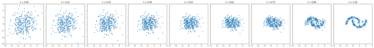
実際にサンプリングしたノイズから三日月データの生成過程を見ると以下のようになります。
x = torch.randn(300, 2)
# t=0からt=1まで8ステップに刻む
n_steps = 8
fig, axes = plt.subplots(1, n_steps + 1, figsize=(30, 4), sharex=True, sharey=True)
time_steps = torch.linspace(0, 1.0, n_steps + 1)

axes[0].scatter(x[:, 0].detach(), x[:, 1].detach(), s=10)
axes[0].set_title(f't = {time_steps[0]:.2f}')
axes[0].set_xlim(-3.0, 3.0)
axes[0].set_ylim(-3.0, 3.0)

for i in range(n_steps):
    # 現在のベクトルと次の時刻tを入力し、学習済みのベクトル場に従って次の地点までxが進む
    x = flow.step(x, float(time_steps[i]), float(time_steps[i + 1]))
    axes[i + 1].scatter(x[:, 0].detach(), x[:, 1].detach(), s=10)
    axes[i + 1].set_title(f't = {time_steps[i + 1]:.2f}')

plt.tight_layout()
plt.show()
π0のaction_expert部分を見る
openpiのレポジトリでは以下のあたりにあります。
今回はVLM側には触れず、action_expertの部分だけ見たいので、必要な実装だけ抜き出してサンプルデータで動きを見ていこうと思います。
実装
最後に全体コードを貼りますが、長くなるので説明のため必要な部分だけを記載しています。
本家実装を見つつ、claude codeと対話しつつ、action expertの部分だけ抜き出しました。気づいたら三日月サンプルから急にややこしくなってしまってました...
コード内のコメントでも何をしているのかを補足していきます。
action expertで使う諸々
ここはaction expert特有のものでもないので割愛していきます。
@dataclass
class Pi0ActionConfig:
    """適当な設定"""

    # モデル
    hidden_dim: int = 1024
    num_layers: int = 18
    mlp_dim: int = 4096
    num_heads: int = 8
    num_kv_heads: int = 1
    head_dim: int = 256

    # アクション
    action_dim: int = 32  # 32個の制御対象
    action_horizon: int = 50  # 50ステップ先まで出力

    # 時間埋め込み
    time_min_period: float = 4e-3
    time_max_period: float = 4.0


    dropout: float = 0.0
    rope_theta: float = 10000.0

    @property
    def num_kv_groups(self) -> int:
        return self.num_heads // self.num_kv_heads


class ActionExpertAttention(nn.Module):
    def __init__(self, config: Pi0ActionConfig, layer_idx: int):
        super().__init__()
        (action expertと直接関係ない普通のattentionなので割愛)

    def forward(
        self,
        hidden_states: Tensor,
        attention_mask: Optional[Tensor] = None,
        position_ids: Optional[Tensor] = None,
        cos: Optional[Tensor] = None,
        sin: Optional[Tensor] = None,
    ) -> Tensor:
        """Forward pass

        Args:
            hidden_states: [batch, seq, hidden_dim]
            attention_mask: [batch, 1, seq, seq] (0 = attend, -inf = mask)
            position_ids: [batch, seq]
            cos, sin: RoPE用 [batch, seq, 1, head_dim]
        Returns:
            [batch, seq, hidden_dim]
        """
       (省略)


class ActionExpertMLP(nn.Module):
    def __init__(self, config: Pi0ActionConfig):
        super().__init__()
        self.gate_proj = nn.Linear(config.hidden_dim, config.mlp_dim, bias=False)
        self.up_proj = nn.Linear(config.hidden_dim, config.mlp_dim, bias=False)
        self.down_proj = nn.Linear(config.mlp_dim, config.hidden_dim, bias=False)
        self.act_fn = nn.GELU(approximate="tanh")

    def forward(self, x: Tensor) -> Tensor:
        return self.down_proj(self.act_fn(self.gate_proj(x)) * self.up_proj(x))


class ActionExpertLayer(nn.Module):
    """Action Expert 1層分"""

    def __init__(self, config: Pi0ActionConfig, layer_idx: int):
        super().__init__()
        self.config = config

        self.input_layernorm = RMSNorm(config.hidden_dim)
        self.post_attention_layernorm = RMSNorm(config.hidden_dim)
        self.self_attn = ActionExpertAttention(config, layer_idx)
        self.mlp = ActionExpertMLP(config)

    def forward(
        self,
        hidden_states: Tensor,
        attention_mask: Optional[Tensor] = None,
        position_ids: Optional[Tensor] = None,
        cos: Optional[Tensor] = None,
        sin: Optional[Tensor] = None,
    ) -> Tensor:
        (Attention1層分の計算のみ)
action expert本体
ここがVLMなしで動くaction expertの本体です。とはいえ、基本的には普通のTransformerと同じです。
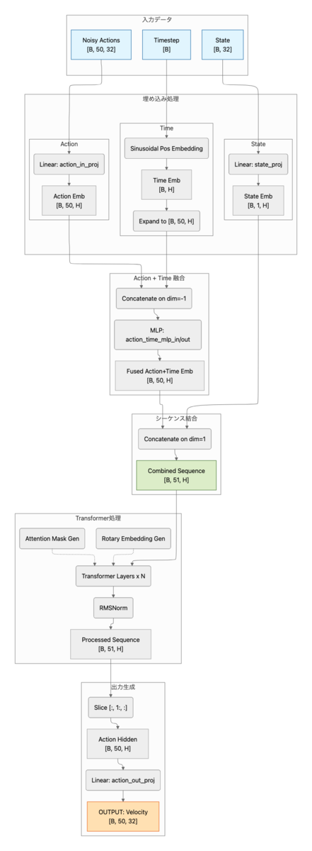
ロボットの現在状態とノイズが混ざったアクションと時間を受け取って、アクションをどの方向に修正していくかを出力します。
embed_suffixでは、まず、時間とアクションの埋め込みをMLPで混ぜ込み、アクショントークンに時間の概念を持たせます。
その後状態トークンとアクショントークンを結合してsuffix_embを作成します。
attention_maskでは、状態トークンは自分以外はmaskされており、各アクショントークンは状態含む全てのトークンを見ることができるようなmaskを作成しています。
それぞれのトークンをtransformerに突っ込み、最後に状態トークンの出力を捨てます。残ったアクショントークン(action_hidden)からアクション次元分の速度(方向)を出力するといった流れです。
class ActionExpert(nn.Module):
    """
    VLMなしで動作する単体のaction expert

    入力:
    - state: [B, 32] ロボット状態
    - noisy_actions: [B, 50, 32] ノイズ付きアクション
    - timestep: [B] Flow Matchingのタイムステップ

    出力:
    - velocity: [B, 50, 32] 予測されたベクトル場
    """

    def __init__(self, config: Pi0ActionConfig):
        super().__init__()
        self.config = config

        self.state_proj = nn.Linear(config.action_dim, config.hidden_dim)
        self.action_in_proj = nn.Linear(config.action_dim, config.hidden_dim)

        # アクション + 時間のMLP融合
        self.action_time_mlp_in = nn.Linear(
            2 * config.hidden_dim, config.hidden_dim
        )
        self.action_time_mlp_out = nn.Linear(config.hidden_dim, config.hidden_dim)

        # RoPE
        self.rotary_emb = RotaryEmbedding(
            config.head_dim,
            max_seq_len=config.action_horizon + 10,
            theta=config.rope_theta,
        )

        # Transformer層
        self.layers = nn.ModuleList(
            [ActionExpertLayer(config, i) for i in range(config.num_layers)]
        )

        # 正規化
        self.norm = RMSNorm(config.hidden_dim)

        # 出力
        self.action_out_proj = nn.Linear(config.hidden_dim, config.action_dim)

    def embed_suffix(
        self,
        state: Tensor,
        noisy_actions: Tensor,
        timestep: Tensor,
    ) -> Tuple[Tensor, Tensor]:
        """suffixトークンを埋め込み
        - state_emb: [B, 1, hidden_dim]
        - action_emb: [B, action_horizon, hidden_dim] + time_emb
        - suffix: [B, 1 + action_horizon, hidden_dim]

        Args:
            state: [batch, action_dim]
            noisy_actions: [batch, action_horizon, action_dim]
            timestep: [batch]
        Returns:
            suffix_emb: [batch, 1 + action_horizon, hidden_dim]
            attention_mask: [batch, 1, seq, seq]

        Note:
             アクションを時間情報を入れて埋め込む
              π0論文の付録Bに記載がある部分
        """
        batch_size = state.shape[0]
        device = state.device

        # 状態埋め込み [batch, 1, hidden_dim]
        state_emb = self.state_proj(state).unsqueeze(1)

        # 時間埋め込み [batch, hidden_dim]
        time_emb = create_sinusoidal_pos_embedding(
            timestep,
            self.config.hidden_dim,
            self.config.time_min_period,
            self.config.time_max_period,
        )

        # アクション埋め込み [batch, action_horizon, hidden_dim]
        action_emb = self.action_in_proj(noisy_actions)

        # アクション + 時間をMLP
        time_emb_expanded = time_emb[:, None, :].expand_as(action_emb)
        action_time_emb = torch.cat([action_emb, time_emb_expanded], dim=-1)
        action_time_emb = self.action_time_mlp_in(action_time_emb)
        action_time_emb = F.silu(action_time_emb)
        action_time_emb = self.action_time_mlp_out(action_time_emb)

        # 結合する [batch, 1 + action_horizon, hidden_dim]
        suffix_emb = torch.cat([state_emb, action_time_emb], dim=1)

        # Attention Mask構築(あっているはず...)
        # att_masks = [1] (状態) + [1] + [0]*(action_horizon-1) (アクション)
        # 1 = 新しいブロックの開始(前のトークンはこれ以降を見れない)
        # 0 = 同じブロック内(双方向Attention)
        seq_len = suffix_emb.shape[1]  # 1 + action_horizon
        att_pattern = torch.zeros(seq_len, dtype=torch.long, device=device)
        att_pattern[0] = 1  # 状態トークン: 新ブロック
        att_pattern[1] = 1  # アクション最初のトークン: 新ブロック

        cumsum = torch.cumsum(att_pattern, dim=0)
        att_2d = cumsum[None, :] <= cumsum[:, None]  # [seq, seq]
        attention_mask = att_2d[None, None, :, :].expand(batch_size, 1, seq_len, seq_len)
        attention_mask = torch.where(
            attention_mask,
            torch.zeros_like(attention_mask, dtype=suffix_emb.dtype),
            torch.full_like(attention_mask, float("-inf"), dtype=suffix_emb.dtype),
        )

        return suffix_emb, attention_mask

    def forward(
        self,
        state: Tensor,
        noisy_actions: Tensor,
        timestep: Tensor,
    ) -> Tensor:
        """Forward pass

        Args:
            state: [batch, action_dim]
            noisy_actions: [batch, action_horizon, action_dim]
            timestep: [batch]
        Returns:
            予測されたベクトル場 [batch, action_horizon, action_dim]
        """
        # 入力埋め込み
        hidden_states, attention_mask = self.embed_suffix(state, noisy_actions, timestep)

        batch_size, seq_len, _ = hidden_states.shape

        # Position IDs
        position_ids = torch.arange(seq_len, device=hidden_states.device)
        position_ids = position_ids[None, :].expand(batch_size, -1)

        # RoPE
        cos, sin = self.rotary_emb(hidden_states, position_ids)

        # Transformer層
        for layer in self.layers:
            hidden_states = layer(
                hidden_states,
                attention_mask=attention_mask,
                position_ids=position_ids,
                cos=cos,
                sin=sin,
            )

        # 正規化
        hidden_states = self.norm(hidden_states)

        # 状態トークンを除いてアクション部分のみ取得
        action_hidden = hidden_states[:, 1:, :]

        # ベクトル場(velocity field)の予測
        velocity = self.action_out_proj(action_hidden)

        return velocity
Flow Matching
以下あたりに記載のあるFlow Matching部分だけを抜き取ったものです。
三日月を学習した時と同様に、ノイズからアクションに向かう方向を学習させていきます。
openpiの実装では三日月の時とは逆で、時刻1がノイズで時刻0がアクションになります。 1→0の中間状態をモデルに入力し、ノイズ空間からアクション空間への直線的な経路(u_t)を目標に学習します。
Euler積分は現在地(x_t)と進む方向(v_t)がわかっている時に、stepを刻みながら徐々に進んでいくだけです。
今回のコードだと10stepにしているので、1→0に0.1刻みで進んでいきます。時間の刻み幅dtが負の値なので、x_t = x_t + dt × 速度という式で、速度の逆方向に進んでいきます。
ちなみに僕はなんでopenpiの実装が1→0にしているのかはわかりませんでした。どなたか分かる方いたら教えてください。。。
def sample_noise(shape: Tuple[int, ...], device: torch.device) -> Tensor:
    return torch.randn(shape, device=device)


def sample_time(batch_size: int, device: torch.device) -> Tensor:
    """Beta(1.5, 1.0)分布からtimestepをサンプリング

    openpiではtime = beta * 0.999 + 0.001として
    [0.001, 1.0]の範囲に収める。

    """
    beta_dist = torch.distributions.Beta(1.5, 1.0)
    time = beta_dist.sample((batch_size,)).to(device)
    time = time * 0.999 + 0.001  # [0.001, 1.0]
    return time


def flow_matching_loss(
    model: ActionExpert,
    state: Tensor,
    actions: Tensor,
    noise: Optional[Tensor] = None,
    time: Optional[Tensor] = None,
) -> Tensor:
    """Flow Matching訓練損失

    - x_t = t * noise + (1-t) * actions
    - u_t = noise - actions (target velocity)
    - v_t = model(x_t, t) (predicted velocity)
    - loss = MSE(v_t, u_t)

    Args:
        model: ActionExpertモデル
        state: [batch, action_dim]
        actions: [batch, action_horizon, action_dim]
        noise: オプションのノイズ
        time: オプションのタイムステップ
    Returns:
        [batch, action_horizon, action_dim] の損失
    """
    batch_size = state.shape[0]
    device = state.device

    if noise is None:
        noise = sample_noise(actions.shape, device)
    if time is None:
        time = sample_time(batch_size, device)

    # ノイズ混合: x_t = t * noise + (1-t) * actions
    t = time[:, None, None]  # [batch, 1, 1]
    x_t = t * noise + (1 - t) * actions

    # 予測ターゲット: u_t = noise - actions
    u_t = noise - actions

    # モデル予測
    v_t = model(state, x_t, time)

    # MSE損失
    loss = F.mse_loss(v_t, u_t, reduction="none")

    return loss


@torch.no_grad()
def sample_actions(
    model: ActionExpert,
    state: Tensor,
    num_steps: int = 10,
    noise: Optional[Tensor] = None,
) -> Tensor:
    """Euler積分によるアクション生成

    t=1.0からt=0.0へ逆方向に積分。

    x_{t-dt} = x_t + dt * v_theta(x_t, t)


    Args:
        model: ActionExpertモデル
        state: [batch, action_dim]
        num_steps: 積分ステップ数
        noise: 初期ノイズ(Noneの場合はサンプリング)
    Returns:
        生成されたアクション [batch, action_horizon, action_dim]

    Note:
         openpi実装では1→0の方向で推論
    """
    batch_size = state.shape[0]
    device = state.device
    config = model.config

    # 初期ノイズ
    if noise is None:
        noise = sample_noise(
            (batch_size, config.action_horizon, config.action_dim), device
        )

    # タイムステップ: 1.0 → 0.0
    dt = -1.0 / num_steps
    x_t = noise.clone()
    time = torch.tensor(1.0, device=device)

    # Euler積分
    for _ in range(num_steps):
        timestep = time.expand(batch_size)
        v_t = model(state, x_t, timestep)
        x_t = x_t + dt * v_t
        time = time + dt

    return x_t
サンプルデータを投入して流れを見る
colabのA100で実行していきます。colabで全コード公開しています。本ブログ内では適宜省略して記載していきます。
"""スタンドアロンデモ実行"""
print("\n" + "=" * 60)
print("Pi0 Action Expert Demo (Standalone)")
print("=" * 60)

# デバイス設定
device, dtype = get_device_and_dtype()
print(f"\nDevice: {device}, dtype: {dtype}")

# 設定
config = Pi0ActionConfig()

# モデル作成
print("\nCreating model...")
model = ActionExpert(config).to(device).to(dtype)
print_model_info(model)

# サンプルデータ
batch_size = 2
state = torch.randn(batch_size, config.action_dim, device=device, dtype=dtype)
actions = torch.randn(
    batch_size, config.action_horizon, config.action_dim, device=device, dtype=dtype
)

print("\nSample data:")
print(f"  state shape: {state.shape}")
print(f"  actions shape: {actions.shape}")
============================================================
Pi0 Action Expert Demo (Standalone)
============================================================

Device: cuda, dtype: torch.bfloat16

Creating model...
============================================================
Pi0 Action Expert Model Info
============================================================
Architecture (gemma_300m equivalent):
  hidden_dim: 1024
  num_layers: 18
  mlp_dim: 4096
  num_heads: 8
  num_kv_heads: 1 (GQA)
  head_dim: 256
Action settings:
  action_dim: 32
  action_horizon: 50
Time embedding:
  min_period: 0.004
  max_period: 4.0
Parameters: 314,713,120 (314.7M)
============================================================

Sample data:
  state shape: torch.Size([2, 32])
  actions shape: torch.Size([2, 50, 32])
何も学習せずとりあえずfowardだけしてみます。action horizon(50個)の各時点、各アクション次元(32個)について、ノイズ→真のアクションへ向かう速度ベクトルを予測するので、モデル出力はactionのshapeと同じになります。
# Forward pass テスト
print("\n" + "-" * 40)
print("Forward Pass Test")
print("-" * 40)

model.eval()
with torch.no_grad():
    timestep = torch.tensor([0.5, 0.3], device=device, dtype=dtype)
    velocity = model(state, actions, timestep)
    print(f"Output velocity shape: {velocity.shape}")
----------------------------------------
Forward Pass Test
----------------------------------------
Output velocity shape: torch.Size([2, 50, 32])
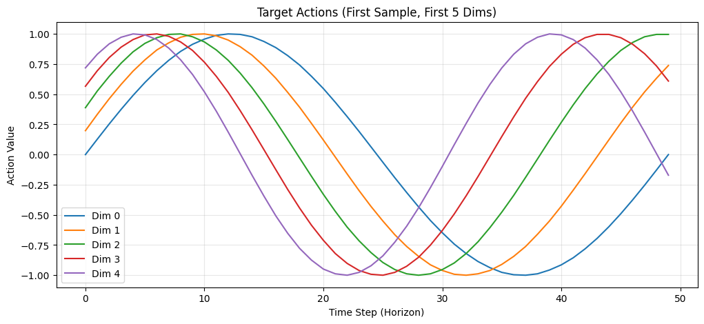
次にFlow Matchingの学習テストをします。目標はなんでもいいので適当にサイン波にしました。
# Flow Matching学習テスト
print("\n" + "-" * 40)
print("Flow Matching Training Test")
print("-" * 40)

# 目標データの作成: サイン波パターン
# 各アクション次元が異なる周波数のサイン波になるようにする
t_horizon = torch.linspace(0, 2 * np.pi, config.action_horizon, device=device)
target_actions = torch.zeros(batch_size, config.action_horizon, config.action_dim, device=device, dtype=dtype)
for d in range(config.action_dim):
    freq = 1 + d * 0.1  # 次元ごとに異なる周波数
    phase = d * 0.2     # 次元ごとに異なる位相
    target_actions[:, :, d] = torch.sin(freq * t_horizon + phase)

print(f"Target actions shape: {target_actions.shape}")
print(f"Target actions range: [{target_actions.min().item():.2f}, {target_actions.max().item():.2f}]")
実際に学習していきましょう。ランダムノイズと目標アクションの間を補間した中間状態 x_t を入力し、正解の速度ベクトル u_t = noise - actions を予測できるようMSE損失で学習します。
# 学習設定
optimizer = torch.optim.AdamW(model.parameters(), lr=1e-4)
num_epochs = 1000

model.train()
losses = []

print(f"\nTraining for {num_epochs} epochs...")
for epoch in range(num_epochs):
    optimizer.zero_grad()

    # Flow Matching損失を計算
    loss = flow_matching_loss(model, state, target_actions)
    loss_mean = loss.mean()

    # 逆伝播
    loss_mean.backward()
    optimizer.step()

    losses.append(loss_mean.item())

    if (epoch + 1) % 20 == 0:
        print(f"  Epoch {epoch + 1:3d}: Loss = {loss_mean.item():.4f}")

print(f"\nTraining completed!")
print(f"  Initial loss: {losses[0]:.4f}")
print(f"  Final loss: {losses[-1]:.4f}")
Training for 1000 epochs...
  Epoch  20: Loss = 1.5312
  Epoch  40: Loss = 1.5469
  Epoch  60: Loss = 1.4609
  Epoch  80: Loss = 1.0625
  Epoch 100: Loss = 0.9961
(省略)
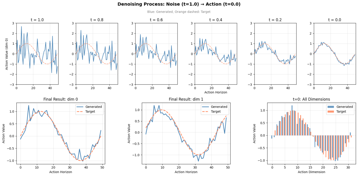
学習したモデルで推論していきます。ランダムノイズから始めて、学習した速度場に従いEuler積分で t=1→0 へ10ステップ進め、アクションを生成します。
t=1.0(ノイズ)から t=0.0(アクション)まで10ステップで変化する過程を、初期状態含め11フレーム分記録するので、Trajectory shapeの0次元目は11になります。
# 推論テスト
print("\n" + "-" * 40)
print("Inference Test (Euler Integration)")
print("-" * 40)

model.eval()
num_steps = 10

# 軌跡を記録
initial_noise = sample_noise((1, config.action_horizon, config.action_dim), device).to(dtype)
single_state = state[:1]

# Numpy doesn't support bfloat16, so cast to float32 first
trajectory = [initial_noise.float().cpu().numpy().copy()]
x_t = initial_noise.clone()
time = 1.0
dt = -1.0 / num_steps

with torch.no_grad():
    for step in range(num_steps):
        timestep = torch.tensor([time], device=device, dtype=dtype)
        v_t = model(single_state, x_t, timestep)
        x_t = x_t + dt * v_t
        time = time + dt
        trajectory.append(x_t.float().cpu().numpy().copy())

trajectory = np.array(trajectory)
print(f"Trajectory shape: {trajectory.shape}")

generated_actions = sample_actions(model, single_state, num_steps=num_steps)
print(f"Generated actions shape: {generated_actions.shape}")
----------------------------------------
Inference Test (Euler Integration)
----------------------------------------
Trajectory shape: (11, 1, 50, 32)
Generated actions shape: torch.Size([1, 50, 32])
簡単に推論結果を可視化します。以下のような内容を図にしています。
| 位置 | 内容 |
|---|---|
| 上段 | Denoising過程(t=1.0, 0.8, 0.6, 0.4, 0.2, 0.0 の6フレーム) |
| 下段左 | 生成 vs 目標(dim 0、全horizon) |
| 下段中央 | 生成 vs 目標(dim 1、全horizon) |
| 下段右 | 生成 vs 目標(t=0、全32次元) |
全コードをcolabで
以下に公開しています。上からぽちぽちするだけで動くはずです。 Google Colab
最後に
サンプルデータの流し込みとはいえ、この記事を執筆する前よりはaction expertについて理解を(多少)深めることができました。 特にFlow Matchingの部分はなんとなくの理解にとどまっていましたが、実際のコードとデータの変化を追いかけることで、意外とシンプルな仕組みで動いていることが実感できたのは収穫でした。次は実際のVLAデータで試していければと思います。
We Are Hiring!
ABEJAは、テクノロジーの社会実装に取り組んでいます。 技術はもちろん、技術をどのようにして社会やビジネスに組み込んでいくかを考えるのが好きな方は、下記採用ページからエントリーください! (新卒の方や通年インターンシップのエントリーもお待ちしております!) careers.abejainc.com
特に下記ポジションの募集を強化しています!ぜひ御覧ください!
